Advection-diffusion Problem

Advection-diffusion problems are common in nature. They include mixing of and heat diffusion in fluids.

VelocityCoupling2D

The incompressible Navier-Stokes equations:

$$\partial_t\boldsymbol{u}+(\boldsymbol{u}\cdot\nabla)\boldsymbol{u}=-\frac{1}{\rho_0}\nabla p+\nu\Delta\boldsymbol{u}$$ $$\nabla\cdot\boldsymbol{u} = 0$$

and couple the flow with an advection-diffusion equation (one-way coupling): $$\frac{\partial C}{\partial t}+\boldsymbol{u}\cdot\nabla C=D\nabla^2C$$ For the advection-diffusion equation, the left-hand side describes the advection of C in the presence of an external fluid velocity $\mu$ while the right-hand side contains a diffusion term with diffusion coefficient D.

We use two different lattice descriptors, one for the fluid, and one for the scalar, since they are based on different LBM models:

1
2
3
4
5
6
using namespace plb;
using namespace plb::descriptors;

typedef double T;
#define NS_DESCRIPTOR D2Q9Descriptor
#define AD_DESCRIPTOR AdvectionDiffusionD2Q5Descriptor

And we instantiate two lattices:

1
2
MultiBlockLattice2D<T,NS_DESCRIPTOR>
MultiBlockLattice2D<T,AD_DESCRIPTOR>

The idea for the coupling is:

Write a data processor which, when applied, receives the two lattices. On every lattice cell, it computes the velocity from the fluid lattice, and copies it to the scalar lattice.

In this example: two lattices, the operation to be performed is not reductive. The base data process functional class is the BoxProcessingFunctional2D_LL

Declaration of the data processor:

 1
 2
 3
 4
 5
 6
 7
 8
 9
10
11
template<typename T,
         template<typename U1> class DESCRIPTOR1,
         template<typename U2> class DESCRIPTOR2 >
class VelocityCoupling2D : public BoxProcessingFunctional2D_LL<T, DESCRIPTOR1, T, DESCRIPTOR2>
{
public:
    VelocityCoupling2D() { }
    virtual void process(Box2D domain, BlockLattice2D<T,DESCRIPTOR1>& fluid, BlockLattice2D<T,DESCRIPTOR2>& scalar);
    virtual VelocityCoupling2D<T,DESCRIPTOR1,DESCRIPTOR2>* clone() const;
    virtual void getTypeOfModification(std::vector<modif::ModifT>& modified) const;
};

Implementation of clone function:

All Palabos processing functions have a clone function, which creates an exact copy of a class instantiation:

1
2
3
4
5
6
7
template<typename T,
         template<typename U1> class DESCRIPTOR1,
         template<typename U2> class DESCRIPTOR2 >
VelocityCoupling2D<T,DESCRIPTOR1,DESCRIPTOR2>* VelocityCoupling2D<T,DESCRIPTOR1,DESCRIPTOR2>::clone() const
{
    return new VelocityCoupling2D<T,DESCRIPTOR1,DESCRIPTOR2>(*this);
}

Implementation of getTypeOfModification:

A data processor must also implement getTypeOfModification :

1
2
3
4
5
6
7
8
template<typename T,
         template<typename U1> class DESCRIPTOR1,
         template<typename U2> class DESCRIPTOR2 >
void VelocityCoupling2D<T,DESCRIPTOR1,DESCRIPTOR2>::getTypeOfModification(std::vector<modif::ModifT>& modified) const
{
    modified[0] = modif::nothing;
    modified[1] = modif::staticVariables;
}

The modified argument indicates, for every block, which kind of cell content was modified and needs to be updated. The values it can adopt are the following:

Argument Descriptions
nothing No modification
staticVariables Static cell content (e.g. populations)
dynamicVariables Content of dynamics objects (e.g. relaxation time)
allVariables Both static and dynamic content
dataStructure Recreate dynamics object and copy static data

Implementation of process:

The process method is the actual algorithm.

It is applied repeatedly to rectangular areas on which atomic-blocks of the two fields intersect.

When calling the process method, Palabos provides a domain argument: the coordinates of the domain on which the data processor is executed.

Process Algorithm

The coordinates of the domain are always local to the atomic-block which is passed first as an argument of the process function. Suppose that atomic-block fluid is passed first and atomic-block scalar is passed second. Suppose also that we have a point (iX, iY), in the local coordinates of fluid, with:

1
2
domain.x0 <= iX <= domain.x1
domain.y0 <= iY <= domain.y1

then the coordinates of the same point local to the block scalar will be (iX+offset.x, iY+offset.y), with:

1
Dot2D ofs = computeRelativeDisplacement(fluid, scalar);

To access absolute coordinates, we need to add an offset:

1
2
3
Dot2D location = fluid.getLocation();
plint globalX = iX + location.x;
plint globalY = iY + location.y;

The Palabos code for the implementation of process:

 1
 2
 3
 4
 5
 6
 7
 8
 9
10
11
12
13
14
15
16
template<typename T,
         template<typename U1> class DESCRIPTOR1,
         template<typename U2> class DESCRIPTOR2 >
void VelocityCoupling2D<T,DESCRIPTOR1,DESCRIPTOR2>::process(Box2D domain, BlockLattice2D<T,DESCRIPTOR1>& fluid,                                 BlockLattice2D<T,DESCRIPTOR2>& scalar)
{
	const int velOffset = DESCRIPTOR2<T>::ExternalField::velocityBeginsAt;
	Dot2D ofs = computeRelativeDisplacement(fluid, scalar);
	for (plint iX=domain.x0; iX<=domain.x1; ++iX) {
		for (plint iY=domain.y0; iY<=domain.y1; ++iY) {
            T *u = scalar.get(iX+ofs.x,iY+ofs.y).getExternal(velOffset);
            Array<T,2> velocity;
            fluid.get(iX,iY).computeVelocity(velocity);
            velocity.to_cArray(u);
        }
    }
}

The result of coupled cavity2d is displayed:

Coupled 2D Cavityl Illustration

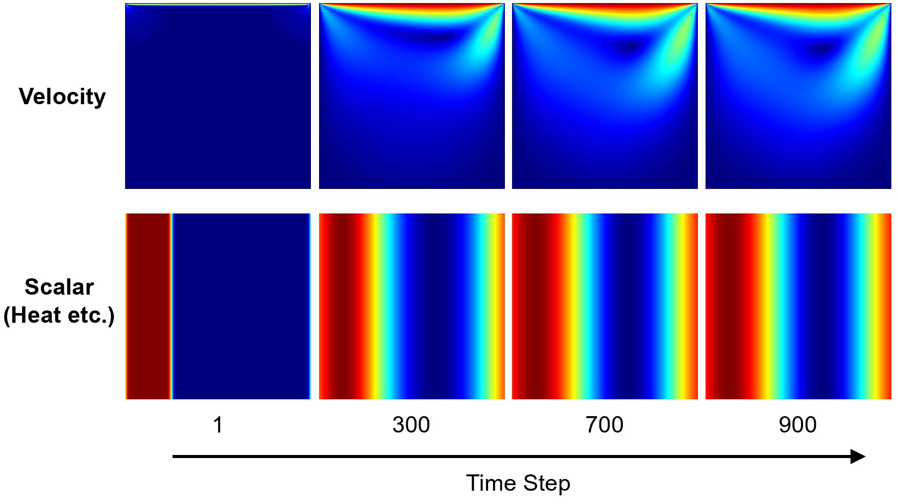
Scalar Field Less Diffusive

The diffusion coefficient D in the BGK model is given by the relaxation time \tau_g, similarity to the viscosity in the NSE: $$ \begin{align*} D={c_s}^2(\tau_g-\frac{\Delta t}{2}) \end{align*} $$ Therefore, to make field less diffusive, them it is need do reduce *D*, which is to reduce \tau_g or increase \omega.

1
    double omega_ad = 1 / 0.51; // 0.60, change from 0.60 to 0.51 to make the field sharper

ApplyProcessingFunctional

Instead of integrating VelocityCoupling2D into ad_lattice, call it manually at every iteration through the function applyProcessingFunctional.

Rules of data processing functionals

  • A data processor acts on a subdomain of all atomic-blocks passed to it.
  • The data processor can write into that subdomain.
  • The data processor can read outside that subdomain, only to an extend given by the communication envelope of the corresponding atomic-block.
  • The operation performed by the data processor can be space dependent, if this dependence is formulated in terms of absolute coordinates.
  • A data processor must always be written in such a way that executing it on a given domain has the same effect as splitting the domain into subdomains, and then executing it consecutively on each of these subdomains.

Applying and integrating data processing functional

Two ways of using a data processor:

  1. Execute the processor only once.
  2. Add the processor to a block and assign to it the role of an internal data processor. The internal data processor can be executed as many times as wished.

To apply the data processor only once, use applyProcessingFunctional:

1
2
3
applyProcessingFunctional (
	new VelocityCoupling<T,D,S_D>, lattice.getBoundingBox(),
	ns_lattice, ad_lattice)

To add a data processor to a specific multi-block, one must integrate the processor, by using the function integrateProcessingFunctional:

1
2
3
integrateProcessingFuncation(
	new Coupling<T,D,S_D>, lattice.getBoundingBox(),
	lattice, s_lattice, level)

In this example, the codes:

1
2
3
4
plint processorLevel = 1;
integrateProcessingFunctional (
    new VelocityCoupling2D<T, NS_DESCRIPTOR, AD_DESCRIPTOR>(), 
    ns_lattice.getBoundingBox(), ns_lattice, ad_lattice, processorLevel );

This way, the processor is added to the multi-block lattice and is executed at processor level .

All internal processor added to a multi-block can be executed at any time by a call to the specific block's method executedInternalProcessors, for a specific processor level.

In a multi-block lattice, internal processors have a special role, since the method executedInternalProcessors is automatically invoked at the end of the method collideAndStream after the streaming step.

For this task, the code for ApplyProcessingFunctional:

1
2
3
	applyProcessingFunctional ( 
			new VelocityCoupling2D<T,NS_DESCRIPTOR, AD_DESCRIPTOR>, ns_lattice.getBoundingBox(), 
			ns_lattice, ad_lattice ); // applyProcessingFunctional-20200708

Data Processor

Execution order of data processors

  • All processor levels are transverse in increasing order starting from level 0.
  • Inside a processor level, the data processors are executed in the order they were added to the block.
  • Communication (update of envelopes) is performed after an execution of a data processor with write access only when switching from one processor level to the next.
  • The processor level can have a negative value. The negative processor level is not executed by the default function executeInternalProcessors(), which executes all non-negatives levels, but must independently executed by a call to the function executeInternalProcessor(plint level).

Reductive data processors: computing an average

Compute the average value of the N cells in a scalar field C: $$C_{av}=\frac{1}{N}\sum_iC_i$$ The Palabos function to compute this average is the following:

template<typename T>
T computeAverage(MultiScalarField3D<T>& scalarField, Box3D domain)
{
	BoxScalarSumFunctional3D<T> functional;
	applyProcessingFuncational(funcational, domain, scalarField);
	reture funcational.getSumScalar() / (T) domain.nCells();
}

It uses the reductive data processor BoxScalarSumFuncional3D.

Declaration of BoxScalarSumFunctional3D

 1
 2
 3
 4
 5
 6
 7
 8
 9
10
11
12
template<typename T>
class BoxScalarSumFunctional3D : public ReductiveBoxProcessingFunctional3D_S<T>
{
public:
	BoxScalarSumFunctional3D();
	virtual void process(Box3D domain, ScalarField3D<T>& scalarField);
	virtual BoxScalarSumFunctional3D<T>* clone() const;
	virtual void getTypeOfModification(std::vector<modif::ModifT>& modified) const
	T getSumScalar() const
private:
	plint sumScalarId;
}

BoxScalarSumFunctional3D::process

 1
 2
 3
 4
 5
 6
 7
 8
 9
10
11
12
13
14
template<typename T>
void BoxScalarSumFunctional3D<T>::process(
	Box3D domain, ScalarField3D<T>& scalarField)
{
    BlockStatics& statistics = this->getStatistics();
    for (plint iX=domain.x0; iX<=domain.x1; ++iX){
        for (plint iY=domain.y0; iY<=domain.y1; ++iY) {
            for (plint iZ=domain.z0; iZ<=domain.z1; ++iZ) {
            statisics.gatherSum(sumScalarId,
                               (double)scalarField.get(iX, iY, iZ));
            }
        }
    }
}

BoxScalarSumFunctional3D

1
2
3
4
template<typename T>
BoxScalarSumFunctional3D<T>::BoxScalarSumFuncational3D()
	: sumScalarId(this->getStatistics().subscribeSum())
{ }
1
2
3
4
template<typename T>
BoxScalarSumFunctional3D<T>::getSumScalar() const {
    return this->getStatistics().getSum(sumScalarId);
}

Boundary Condition for the Scalar Field

see Palabos example BoussinesqThermal2D

GIF Animations

Using gifsicle to generate an animation of GIFs

1
gifsicle --colors 256 --loop *.gif > anim.gif

Full Codes

  1
  2
  3
  4
  5
  6
  7
  8
  9
 10
 11
 12
 13
 14
 15
 16
 17
 18
 19
 20
 21
 22
 23
 24
 25
 26
 27
 28
 29
 30
 31
 32
 33
 34
 35
 36
 37
 38
 39
 40
 41
 42
 43
 44
 45
 46
 47
 48
 49
 50
 51
 52
 53
 54
 55
 56
 57
 58
 59
 60
 61
 62
 63
 64
 65
 66
 67
 68
 69
 70
 71
 72
 73
 74
 75
 76
 77
 78
 79
 80
 81
 82
 83
 84
 85
 86
 87
 88
 89
 90
 91
 92
 93
 94
 95
 96
 97
 98
 99
100
101
102
103
104
105
106
107
108
109
110
111
112
113
114
115
116
117
118
119
120
121
122
123
124
125
126
127
128
129
130
131
132
133
134
135
136
137
138
139
140
141
142
143
144
145
146
147
148
149
150
151
152
153
154
155
156
157
158
159
160
161
162
163
164
165
166
167
168
169
170
171
172
173
174
175
176
177
178
179
180
181
182
183
184
185
186
187
188
189
190
191
192
193
194
195
196
197
198
199
200
201
202
203
204
205
206
207
208
209
210
211
212
213
214
215
216
217
218
219
220
221
222
223
224
225
226
227
228
229
230
231
232
233
234
235
236
237
238
239
240
241
242
243
244
245
246
247
248
249
250
251
252
253
254
255
256
257
258
259
260
261
262
263
264
265
266
267
/* This file is part of the Palabos library.
 *
 * Copyright (C) 2011-2017 FlowKit Sarl
 * Route d'Oron 2
 * 1010 Lausanne, Switzerland
 * E-mail contact: contact@flowkit.com
 *
 * The most recent release of Palabos can be downloaded at
 * <http://www.palabos.org/>
 *
 * The library Palabos is free software: you can redistribute it and/or
 * modify it under the terms of the GNU Affero General Public License as
 * published by the Free Software Foundation, either version 3 of the
 * License, or (at your option) any later version.
 *
 * The library is distributed in the hope that it will be useful,
 * but WITHOUT ANY WARRANTY; without even the implied warranty of
 * MERCHANTABILITY or FITNESS FOR A PARTICULAR PURPOSE.  See the
 * GNU Affero General Public License for more details.
 *
 * You should have received a copy of the GNU Affero General Public License
 * along with this program.  If not, see <http://www.gnu.org/licenses/>.
*/

/** \file
  * Flow in a 2D cavity.
  **/

#include "palabos2D.h"
#include "palabos2D.hh"   // include full template code

#include <vector>
#include <cmath>
#include <iostream>
#include <fstream>
#include <iomanip>

using namespace plb;
using namespace plb::descriptors;

typedef double T;
#define NS_DESCRIPTOR D2Q9Descriptor
#define AD_DESCRIPTOR AdvectionDiffusionD2Q5Descriptor

// Global variables for conveniently passing data in functions.

static plint nx, ny;
static T dx, dt;
static T uLB;

void cavitySetup(MultiBlockLattice2D<T,NS_DESCRIPTOR>& ns_lattice,
        OnLatticeBoundaryCondition2D<T,NS_DESCRIPTOR>& boundaryCondition)
{
    Box2D top(0, nx-1, ny-1, ny-1);
    Box2D bottom(0, nx-1, 0,    0);
    Box2D left(0, 0, 1, ny-2);
    Box2D right(nx-1, nx-1, 1, ny-2);

    boundaryCondition.setVelocityConditionOnBlockBoundaries(ns_lattice, top);
    boundaryCondition.setVelocityConditionOnBlockBoundaries(ns_lattice, bottom);
    boundaryCondition.setVelocityConditionOnBlockBoundaries(ns_lattice, left);
    boundaryCondition.setVelocityConditionOnBlockBoundaries(ns_lattice, right);

    T u = uLB;
    setBoundaryVelocity(ns_lattice, top, Array<T,2>(u,(T)0.) );
    setBoundaryVelocity(ns_lattice, bottom, Array<T,2>((T)0.,(T)0.) );
    setBoundaryVelocity(ns_lattice, left, Array<T,2>((T)0.,(T)0.) );
    setBoundaryVelocity(ns_lattice, right, Array<T,2>((T)0.,(T)0.) );

    initializeAtEquilibrium(ns_lattice, ns_lattice.getBoundingBox(), (T)1., Array<T,2>((T)0.,(T)0.) );
    initializeAtEquilibrium(ns_lattice, top, (T)1., Array<T,2>(u,(T)0.) );

    ns_lattice.initialize();
}

void writePpm(MultiBlockLattice2D<T,NS_DESCRIPTOR>& ns_lattice, MultiBlockLattice2D<T,AD_DESCRIPTOR>& ad_lattice, plint iter)
{
    static plint iFile = 0;

    // iFile = iter;
    ImageWriter<T> imageWriter("leeloo");
    imageWriter.writeScaledPpm(createFileName("uNorm", iFile, 6), *computeVelocityNorm(ns_lattice));
    imageWriter.writeScaledPpm(createFileName("logUnorm", iFile, 6),
            *computeLog(*add((T)1.e-8,*computeVelocityNorm(ns_lattice))));
    imageWriter.writeScaledPpm(createFileName("scalar", iFile, 6), *computeDensity(ad_lattice));

    iFile++;
}

template<class BlockLatticeT>
void writeVTK(BlockLatticeT& ns_lattice, plint iter)
{
    static plint iFile = 0;

    // iFile = iter;
    VtkImageOutput2D<T> vtkOut(createFileName("vtk", iFile, 6), dx);
    vtkOut.writeData<float>(*computeVelocityNorm(ns_lattice), "velocityNorm", dx/dt);
    vtkOut.writeData<2,float>(*computeVelocity(ns_lattice), "velocity", dx/dt);

    iFile++;
}

template<typename T,
         template<typename U1> class DESCRIPTOR1,
         template<typename U2> class DESCRIPTOR2 >
class VelocityCoupling2D : public BoxProcessingFunctional2D_LL<T, DESCRIPTOR1, T, DESCRIPTOR2>
{
public:
    VelocityCoupling2D() { }
    virtual void process(Box2D domain, BlockLattice2D<T,DESCRIPTOR1>& fluid, BlockLattice2D<T,DESCRIPTOR2>& scalar);
    virtual VelocityCoupling2D<T,DESCRIPTOR1,DESCRIPTOR2>* clone() const;
    virtual void getTypeOfModification(std::vector<modif::ModifT>& modified) const;
};

template<typename T,
         template<typename U1> class DESCRIPTOR1,
         template<typename U2> class DESCRIPTOR2 >
void VelocityCoupling2D<T,DESCRIPTOR1,DESCRIPTOR2>::process(Box2D domain, BlockLattice2D<T,DESCRIPTOR1>& fluid,
                                                                          BlockLattice2D<T,DESCRIPTOR2>& scalar)
{
	const int velOffset = DESCRIPTOR2<T>::ExternalField::velocityBeginsAt;
	Dot2D ofs = computeRelativeDisplacement(fluid, scalar);
	for (plint iX=domain.x0; iX<=domain.x1; ++iX) {
		for (plint iY=domain.y0; iY<=domain.y1; ++iY) {
            T *u = scalar.get(iX+ofs.x,iY+ofs.y).getExternal(velOffset);
            Array<T,2> velocity;
            fluid.get(iX,iY).computeVelocity(velocity);
            velocity.to_cArray(u);
        }
    }
}

template<typename T,
         template<typename U1> class DESCRIPTOR1,
         template<typename U2> class DESCRIPTOR2 >
VelocityCoupling2D<T,DESCRIPTOR1,DESCRIPTOR2>* VelocityCoupling2D<T,DESCRIPTOR1,DESCRIPTOR2>::clone() const
{
    return new VelocityCoupling2D<T,DESCRIPTOR1,DESCRIPTOR2>(*this);
}


template<typename T,
         template<typename U1> class DESCRIPTOR1,
         template<typename U2> class DESCRIPTOR2 >
void VelocityCoupling2D<T,DESCRIPTOR1,DESCRIPTOR2>::getTypeOfModification(std::vector<modif::ModifT>& modified) const
{
    modified[0] = modif::nothing;
    modified[1] = modif::staticVariables;
}

int main(int argc, char* argv[])
{
    plbInit(&argc, &argv);

    global::directories().setOutputDir("./tmp/");

    // Physical parameters (chosen by the user).

    T lx = 0.05;
    T ly = 0.05;
    T uPhys = 0.02;
    T nuPhys = 0.00001;

    // Numerical parameters (need to be filled by the participants).

    uLB = 0.01;
    plint N = 256;

    dx = lx / ((T) N - 1);
    nx = util::roundToInt(lx / dx) + 1;
    ny = util::roundToInt(ly / dx) + 1;

    dt = dx * uLB / uPhys;

    T nuLB = nuPhys * dt / (dx * dx);

    T tau = NS_DESCRIPTOR<T>::invCs2 * nuLB + 0.5;
    T omega = 1.0 / tau;

    // Iteration intervals for output and end of the simulation

    plint logIter   = 50;
    plint imIter    = 100;
    plint vtkIter   = 500;
    plint maxIter   = 100000;

    // Print key parameters.

    pcout << "dx = " << dx << std::endl;
    pcout << "nx = " << nx << std::endl;
    pcout << "ny = " << ny << std::endl;
    pcout << "dt = " << dt << std::endl;
    pcout << "nuPhys = " << nuPhys << std::endl;
    pcout << "nuLB = " << nuLB << std::endl;
    pcout << "tau = " << tau << std::endl;
    pcout << "omega = " << omega << std::endl;
    pcout << "Re = " << uPhys * lx / nuPhys << std::endl;

    double omega_ad = 1 / 0.6;

    MultiBlockLattice2D<T, NS_DESCRIPTOR> ns_lattice (
              nx, ny,
              new BGKdynamics<T,NS_DESCRIPTOR>(omega) );

    MultiBlockLattice2D<T, AD_DESCRIPTOR> ad_lattice (
              nx, ny,
              new AdvectionDiffusionBGKdynamics<T,AD_DESCRIPTOR>(omega_ad) );
    ad_lattice.periodicity().toggleAll(true);


    plint processorLevel = 1;
    integrateProcessingFunctional (
            new VelocityCoupling2D<T, NS_DESCRIPTOR, AD_DESCRIPTOR>(), 
            ns_lattice.getBoundingBox(), ns_lattice, ad_lattice, processorLevel );

    Box2D leftDomain(ad_lattice.getBoundingBox());
    leftDomain.x1 = leftDomain.x1 / 4;
    initializeAtEquilibrium(ad_lattice, leftDomain, 2.0, Array<T,2>(0.,0.));
    ad_lattice.initialize();

    OnLatticeBoundaryCondition2D<T,NS_DESCRIPTOR>*
        boundaryCondition = createLocalBoundaryCondition2D<T,NS_DESCRIPTOR>();

    cavitySetup(ns_lattice, *boundaryCondition);

    T previousIterationTime = T();

    // Main loop over time iterations.
    for (plint iT=0; iT<maxIter; ++iT) {
        global::timer("mainLoop").restart();

        if (iT%imIter==0) {
            pcout << "Saving PPM image ..." << std::endl;
            writePpm(ns_lattice, ad_lattice, iT);
            pcout << std::endl;
        }

        if (iT%vtkIter==0) {
            pcout << "Saving VTK file ..." << std::endl;
            writeVTK(ns_lattice, iT);
        }

        if (iT%logIter==0) {
            pcout << "step " << iT
                  << "; t=" << iT*dt;
        }

        // Lattice Boltzmann iteration step.
        ad_lattice.collideAndStream();
        ns_lattice.collideAndStream();

        if (iT%logIter==0) {
            pcout << "; av energy="
                  << std::setprecision(10) << getStoredAverageEnergy(ns_lattice)
                  << "; av rho="
                  << getStoredAverageDensity(ns_lattice) << std::endl;
            pcout << "Time spent during previous iteration: "
                  << previousIterationTime << std::endl;
        }

        previousIterationTime = global::timer("mainLoop").stop();
    }

    delete boundaryCondition;

    return 0;
}
updatedupdated2020-08-282020-08-28